Build Your Own Llama 3 Architecture

Written by Milan Tamang
Source: https://pub.towardsai.net/build-your-own-llama-3-architecture-from-scratch-using-pytorch-2ce1ecaa901c

A step-by-step guide to building the complete architecture of the Llama 3 model from scratch and performing training and inferencing on a custom dataset.

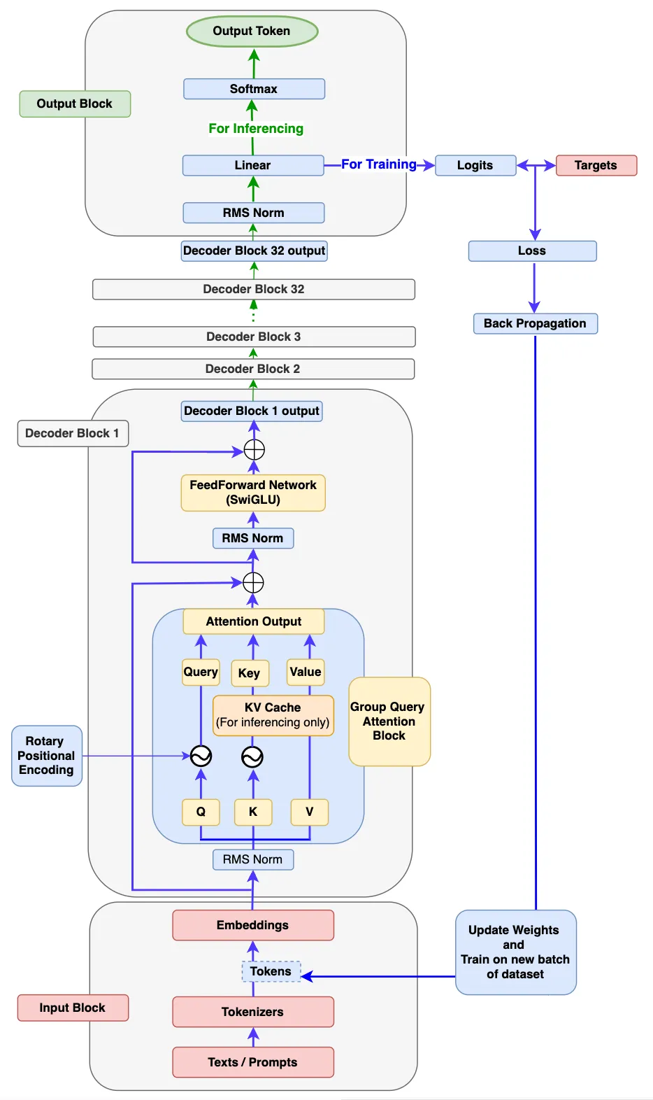
Llama 3 architecture shows training and inferencing flow. I imagined this diagram as the official Llama 3 paper doesn’t have one. By the end of this article, I believe you should be able to draw a better architecture than this one.

What will you achieve by the end of this article?

1. You’ll get an in-depth intuition of how each component of the Llama 3 model works under the hood.
2. You’ll write codes to build each component of Llama 3 and then assemble them all together to build a fully functional Llama 3 model.
3. You’ll also write codes to train your model with new custom datasets.
4. You’ll also write code to perform inferencing so that your Llama 3 model can generate new texts based on input prompts.

Prerequisites

A basic knowledge of Python and Pytorch is required. A basic understanding of transformer concepts such as Self- attention and also knowledge of deep neural networks would certainly help though not compulsory.

Now that we know what we want to achieve, let’s start building everything step by step.

Step 1: The Input Block

As shown in the Llama 3 architecture diagram above, the input block has 3 components:- Texts/ Prompts, Tokenizer and Embeddings.

How do the components inside the Input Block work? There is a popular saying “A picture is worth a thousand words”, let’s check the flow diagram below to understand the workflow inside the Input block.

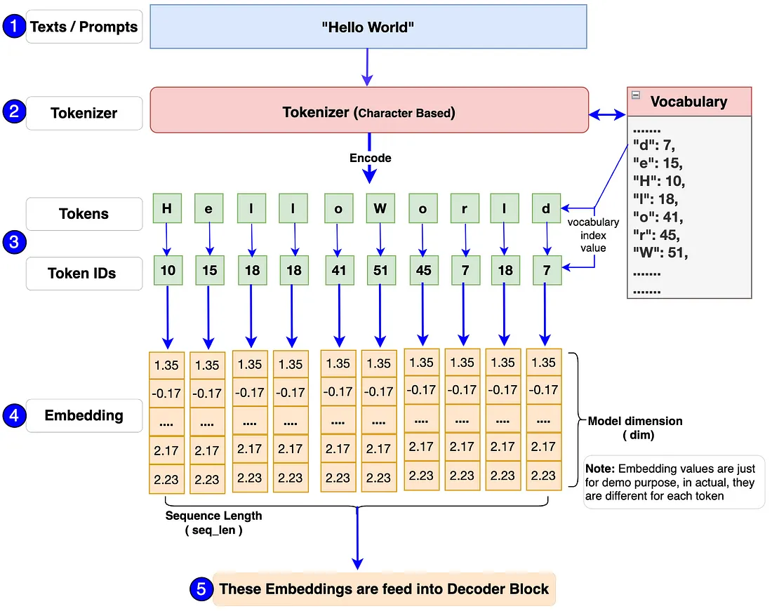
First of all, a single or batch of texts/prompts will be passed into the model. For example: “Hello World” in the above flow diagram.

The input to the model should always be in number format as it is unable to process text. Tokenizer helps to convert these texts/prompts into token-ids (which is an index number representation of tokens in vocabulary). We’ll use the popular Tiny Shakespeare dataset to build the vocabulary and also train our model.

The tokenizer used in the Llama 3 model is TikToken, a type of subword tokenizer. However, we’ll be using a character-level tokenizer for our model building. The main reason is that we should know how to build a vocabulary and tokenizer including encode and decode functions all by ourselves. This way we’ll be able to learn how everything works under the hood and we’ll have full control over the code.

Finally, each token-id will be transformed into an embedding vector of dimensions 128 (in original Llama 3 8B, it is 4096). The embeddings will then be passed into the next block called the Decoder Block.

# Import necessary libraries
import torch
from torch import nn
from torch.nn import functional as F

import math
import numpy as np
import time
from dataclasses import dataclass
from typing import Optional, Tuple, List
import pandas as pd
from matplotlib import pyplot as plt

### Step 1: Input Block ###

# Using Tiny Shakespeare dataset for character-level tokenizer. Some part of the following character-level tokenizer is referenced from Andrej karpathy's GitHub (https://github.com/karpathy/nanoGPT/blob/master/data/shakespeare_char/prepare.py) which I found is explained very well.
# Load tiny_shakespeare data file (https://github.com/tamangmilan/llama3/blob/main/tiny_shakespeare.txt)

device: str = 'cuda' if torch.cuda.is_available() else 'cpu'   # Assign device to cuda or cpu based on availability

# Load tiny_shakespeare data file.
with open('tiny_shakespeare.txt', 'r') as f:
  data = f.read()

# Prepare vocabulary by taking all the unique characters from the tiny_shakespeare data
vocab = sorted(list(set(data)))

# Training Llama 3 model requires addtional tokens such as <|begin_of_text|>, <|end_of_text|> and <|pad_id|>, we'll add them into vocabulary
vocab.extend(['<|begin_of_text|>','<|end_of_text|>','<|pad_id|>'])
vocab_size = len(vocab)

# Create a mapping between characters with corresponding integer indexes in vocabulary.
# This is important to build tokenizers encode and decode functions.
itos = {i:ch for i, ch in enumerate(vocab)}
stoi = {ch:i for i, ch in enumerate(vocab)}

# Tokenizers encode function: take a string, output a list of integers
def encode(s):
  return [stoi[ch] for ch in s]

# Tokenizers decode function: take a list of integers, output a string
def decode(l):
  return ''.join(itos[i] for i in l)

# Define tensor token variable to be used later during model training
token_bos = torch.tensor([stoi['<|begin_of_text|>']], dtype=torch.int, device=device)
token_eos = torch.tensor([stoi['<|end_of_text|>']], dtype=torch.int, device=device)
token_pad = torch.tensor([stoi['<|pad_id|>']], dtype=torch.int, device=device)

prompts = "Hello World"
encoded_tokens = encode(prompts)
decoded_text = decode(encoded_tokens)

### Test: Input Block Code ###
# You need take out the triple quotes below to perform testing
"""
print(f"Lenth of shakespeare in character: {len(data)}")
print(f"The vocabulary looks like this: {''.join(vocab)}\n")
print(f"Vocab size: {vocab_size}")
print(f"encoded_tokens: {encoded_tokens}")
print(f"decoded_text: {decoded_text}")
"""
### Test Results: ###
"""
Lenth of shakespeare in character: 1115394
The vocabulary looks like this: 
 !$&',-.3:;?ABCDEFGHIJKLMNOPQRSTUVWXYZabcdefghijklmnopqrstuvwxyz<|begin_of_text|><|end_of_text|><|pad_id|>

Vocab size: 68
encoded_tokens: [20, 43, 50, 50, 53, 1, 35, 53, 56, 50, 42]
decoded_text: Hello World
"""

Step 2: The Decoder Block

If you look at the architecture diagram above, the decoder block consists of the following sub-components.

• RMS Norm
• Rotary Positional Encoding
• KV Cache
• Group Query Attention
• FeedForward Network
• Decoder Block

Let’s deep dive into each of these sub-components one by one.

RMS Norm (Root Mean Square Normalization):

Why do you need RMSNorm? In the architecture diagram above, you must have noticed that the output of the input block i.e. embedding vector passes through the RMSNorm block. This is because the embedding vector has many dimensions (4096 dim in Llama3-8b) and there is always a chance of having values in different ranges. This can cause model gradients to explode or vanish hence resulting in slow convergence or even divergence. RMSNorm brings these values into a certain range which helps to stabilize and accelerate the training process. This makes gradients have more consistent magnitudes and that results in making models converge more quickly.

How does RMSNorm work? Let’s look at the following diagram first.

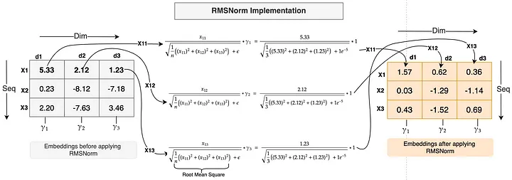
Just like layer normalization, RMSNorm is applied along the embedding features or dimension. The diagram above has embeddings of shape [3,3] meaning each token has 3 dimensions.

Example: Let’s apply RMSNorm to the embedding of the first token X1

• The value of token X1 at each dimension i.e. x11, x12, and x13 will be individually divided by the Root Mean Square of all these values. The formula is shown in the diagram above.
• E (Epsilon) which is a small constant is added to the Root Mean Square to avoid division by Zero for numerical stability.
• Finally, a scaling parameter Gamma (Y) is multiplied by it. Each feature has one unique Gamma parameter (just like Y1 for dim d1, Y2 for dim d2 and Y3 for dim d3 in the diagram above) is a learning parameter that is scaled up or down to bring further stability to the normalization. The gamma parameter is initialized with value 1 (as shown in the calculation above).

As you noticed in the example above, the embedding values are large and spread in a wide range. After applying RMSNorm, the values are much smaller and in a small range. The calculation has been done with actual RMSNorm function.

Why choose RMSNorm over layer normalization? As you noticed above in the example, we didn’t calculate any mean or variance which is done in the case of layer normalization. Thus, we can say that RMSNorm reduces the computational overhead by avoiding the calculation of mean and variance. Also, according to the paper by the Author, RMSNorm gives performance advantages while not compromising on accuracy.

Let’s code the RMSNorm:

# Step2: The Decoder Block
# Note: Since the Llama 3 model is developed by Meta, so to be in sync with their codebase and for future compatibility,
# I will use most of the code from Meta GitHub with some necessary changes required to achieve our goal.

# Define parameters dataclass: we'll use these parameters during model building, training and inference.
# Note: Since we want to see the results of training and inferencing faster rather than focusing on high accuracy, we're taking lower values for most of the parameters which are set higher in the Llama 3 model.

@dataclass
class ModelArgs:
    dim: int = 512              # embedding dimension
    n_layers: int = 8           # number of model decoder blocks
    n_heads: int = 8            # number of heads for queries embedding
    n_kv_heads: int = 4         # number of heads for keys and values embedding
    vocab_size: int = len(vocab) # Length of vocabulary
    multiple_of: int = 256        # Require to calculate dim of feedfoward network
    ffn_dim_multiplier: Optional[float] = None  # Require to calculate dim of feedfoward network
    norm_eps: float = 1e-5                       # Default Epsilon value set for the RMSNorm calculation
    rope_theta: float = 10000.0   # Default theta value for the RePE calculation

    max_batch_size: int = 10     # Max batch size
    max_seq_len: int = 256         # Max sequence length

    epochs: int = 2500             # Total number of training iteration
    log_interval: int = 10        # Number of interval to print the logs and loss values   
    device: str = 'cuda' if torch.cuda.is_available() else 'cpu'   # Assign device to cuda or cpu based on availability 
    
## Step2a: The RMSNorm

class RMSNorm(nn.Module):
  def __init__(self, dim: int, eps: float = 1e-6):
    super().__init__()
    device = ModelArgs.device
    self.eps = eps
    # Scaling parameter gamma, initialized with one and the no of parameters is equal to the size of dim
    self.weight = nn.Parameter(torch.ones(dim).to(device))

  def _norm(self, x):
    return x * torch.rsqrt(x.pow(2).mean(dim=-1, keepdim=True) + self.eps).to(device)

  def forward(self, x):
    #Shape: x[bs,seq,dim]
    output = self._norm(x.float()).type_as(x)

    #Shape: x[bs,seq,dim] -> x_norm[bs,seq,dim]
    return output * self.weight

### Test: RMSNorm Code ###
# You need take out the triple quotes below to perform testing
"""
x = torch.randn((ModelArgs.max_batch_size, ModelArgs.max_seq_len, ModelArgs.dim), device=device)
rms_norm = RMSNorm(dim=ModelArgs.dim)
x_norm = rms_norm(x)

print(f"Shape of x: {x.shape}")
print(f"Shape of x_norm: {x_norm.shape}")
"""
### Test Results: ###
"""
Shape of x: torch.Size([10, 256, 512])
Shape of x_norm: torch.Size([10, 256, 512])
"""    

Rotary Positional Encoding (RoPE):

Why we do need Rotary Positional Encoding (RoPE)? Before we get into the why part, let’s review what we’ve done so far. First, we’ve converted input texts into embeddings. Next, we’ve applied RMSNorm to the embeddings. At this point, you must have noticed something is off. Let’s say the input text is “I love apple” or “apple love I”, the model will still treat both sentences as the same and learn it as the same. Because there is no order defined in the embeddings for the model to learn. Hence, the order is very important for any language model. In Llama 3 model architecture, RePE is used to define the position of each token in the sentences that maintain not only the order but also maintains the relative position of tokens in the sentences.

So, what is Rotary Positional Encoding and how does it work? As mentioned in the why section above, RoPE is a type of position encoding that encodes the embeddings which maintains the order of tokens in the sentences by adding absolute positional information as well as incorporates the relative position information among the tokens. It performs the encoding action by rotating a given embedding by a special matrix called the rotation matrix. This simple yet very powerful mathematical derivation using rotation matrix is the heart of RoPE.

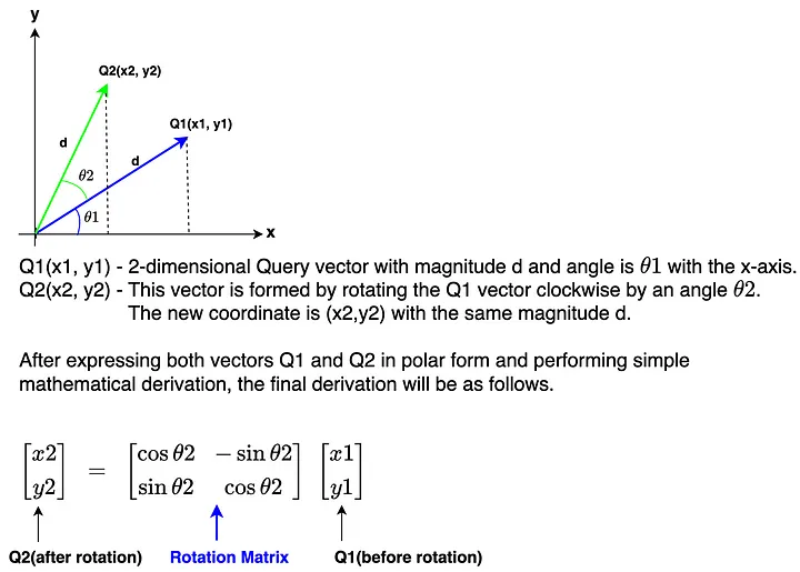
The rotation matrix in the diagram above rotates a vector of 2-dimension. However, the number of dimensions in the Llama 3 model is 4096 which is a lot more. Let’s take a look at how to apply rotation on higher-dimension embeddings.

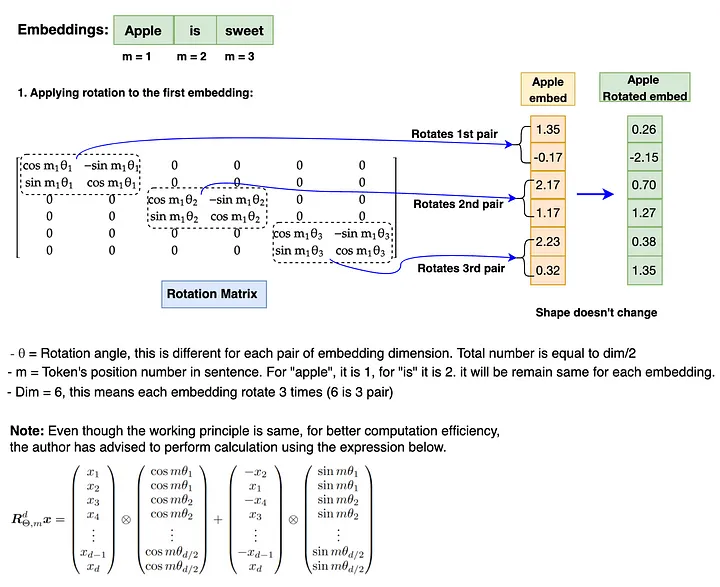
We now know that the rotation of embeddings involves the multiplication of each embedding position (m) value and theta (θ) for each pair of embedding dimensions. This is how RoPE can capture absolute position as well as relative position information by the implementation of the rotation matrix.

Note: the rotation matrix needs to be converted to polar form and the embedding vector needs to be converted to complex before performing rotation. After rotation is completed, the rotated embeddings need to be converted back to real for attention operation. Also, RoPE is applied to Query and Key embedding only. It doesn’t apply to Value embedding.

Let’s dive into RoPE coding:

## Step2b: The RoPE
def precompute_freqs_cis(dim:int, seq_len: int, theta: float=10000.0):
  # Computing Theta value for each dim pair which is dim/2
  device = ModelArgs.device
  freqs = 1.0 / (theta ** (torch.arange(0, dim, 2,device=device)[:(dim//2)].float()/dim))

  # Computing range of positions(m) in the sequence
  t = torch.arange(seq_len, dtype=torch.float32, device=device)

  # freqs gives all the Theta value range for all the position of tokens in the sequence
  freqs = torch.outer(t, freqs).to(device)

  # This is the rotation matrix which needs to be converted to Polar form in order to perform rotation to the embedding
  freqs_cis = torch.polar(torch.ones_like(freqs).to(device), freqs).to(device)
  return freqs_cis

def reshape_for_broadcast(freqs_cis, x):
  ndim = x.ndim
  assert 0<=1Tuple[torch.Tensor, torch.Tensor]:
  device = ModelArgs.device
  # Applying rotary positional encoding to both query and key embedding together
  # First: The last dimension of xq and xk embedding needs to be reshaped to make it a pair. As rotation matrix is applied to each pair of dim.
  # Next: convert both xq and xk to complex number as the rotation matrix is only applicable to complex number
  xq_ = torch.view_as_complex(xq.float().reshape(*xq.shape[:-1], -1, 2)).to(device)    #xq_:[bsz, seq_len, n_heads, head_dim/2]
  xk_ = torch.view_as_complex(xk.float().reshape(*xk.shape[:-1], -1, 2)).to(device)    #xk_:[bsz, seq_len, n_heads, head_dim/2]

  # The rotation matrix(freqs_cis) dimensions across seq_len(dim=1) and head_dim(dim=3) should match with the embedding
  # Also, the shape freqs_cis should be the same with xq and xk, hence change the shape of freqs_cis:[seq_len,head_dim] -> freqs_cis:[1,seq_len,1,head_dim]
  freqs_cis = reshape_for_broadcast(freqs_cis, xq_)

  #Finally, perform rotation operation by multiplying with freqs_cis.
  #After the rotation is completed, convert both xq_out and xk_out back to real number and return
  xq_out = torch.view_as_real(xq_ * freqs_cis).flatten(3).to(device) #xq_out:[bsz, seq_len, n_heads, head_dim]
  xk_out = torch.view_as_real(xk_ * freqs_cis).flatten(3).to(device) #xk_out:[bsz, seq_len, n_heads, head_dim]
  return xq_out.type_as(xq), xk_out.type_as(xk)

### Test: RoPE Code ###
# Note: x_norm is calculated during RMSNorm and is being used for testing here.
# You need take out the triple quotes below to perform testing
"""
head_dim = ModelArgs.dim//ModelArgs.n_heads
wq = nn.Linear(ModelArgs.dim, ModelArgs.n_heads * head_dim, bias=False, device=device)
wk = nn.Linear(ModelArgs.dim, ModelArgs.n_kv_heads * head_dim, bias=False, device=device)
xq = wq(x_norm)
xk = wk(x_norm)
print(f"xq.shape: {xq.shape}")
print(f"xk.shape: {xk.shape}")

xq = xq.view(xq.shape[0],xq.shape[1],ModelArgs.n_heads, head_dim)
xk = xk.view(xk.shape[0],xk.shape[1],ModelArgs.n_kv_heads, head_dim)
print(f"xq.re-shape: {xq.shape}")
print(f"xk.re-shape: {xk.shape}")

freqs_cis = precompute_freqs_cis(dim=head_dim, seq_len=ModelArgs.max_seq_len)
print(f"freqs_cis.shape: {freqs_cis.shape}")

xq_rotate, xk_rotate = apply_rotary_emb(xq, xk, freqs_cis)
print(f"xq_rotate.shape: {xq_rotate.shape}")
print(f"xk_rotate.shape: {xk_rotate.shape}")
"""
### Test Results: ###
"""
xq.shape: torch.Size([10, 256, 512])
xk.shape: torch.Size([10, 256, 256])
xq.re-shape: torch.Size([10, 256, 8, 64])
xk.re-shape: torch.Size([10, 256, 4, 64])
freqs_cis.shape: torch.Size([256, 32])
xq_rotate.shape: torch.Size([10, 256, 8, 64])
xk_rotate.shape: torch.Size([10, 256, 4, 64])
"""

KV Cache (Only required at Inferencing)

What is KV-Cache? In Llama 3 architecture, at the time of inferencing, the concept of KV-Cache is introduced to store previously generated tokens in the form of Key and Value cache. These caches will be used to calculate self-attention to generate the next token. Only key and value tokens are cached whereas query tokens are not cached, hence the term KV Cache.

Why do we need KV Cache? Let’s look at the diagram below to clarify our curiosity.

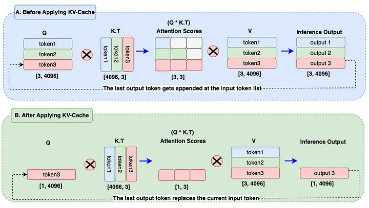
In the A block of the diagram, when the output3 token is being generated, the previous output tokens (output1, output2) are still being calculated which is not necessary at all. This has caused an additional matrix multiplication during attention calculation hence computation resources are increased a lot.

In block B of the diagram, the output tokens replace the input token in Query embedding. KV Cache stores the previously generated tokens. During attention score calculation, we will just have to use 1 token from the query and use previous tokens from the Key and Value cache. It reduces the matrix multiplication from 3x3 to 1x3 from block A to block B, which is almost 66% reduction. In the real world, with huge sequence lengths and batch size, this will help to reduce significant computation power. Finally, there will always be only one latest output token generated. This is the main reason KV-Cache has been introduced.

Group Query Attention

Group query attention is the same as Muilt-Head attention which was used in previous models such as Llama 1 with the only difference being in the use of separate heads for queries and separate heads for keys/values. Usually, the number of heads assigned to queries is n-times to that of keys, and values heads. Let’s take a look at the diagram to build our understanding further.

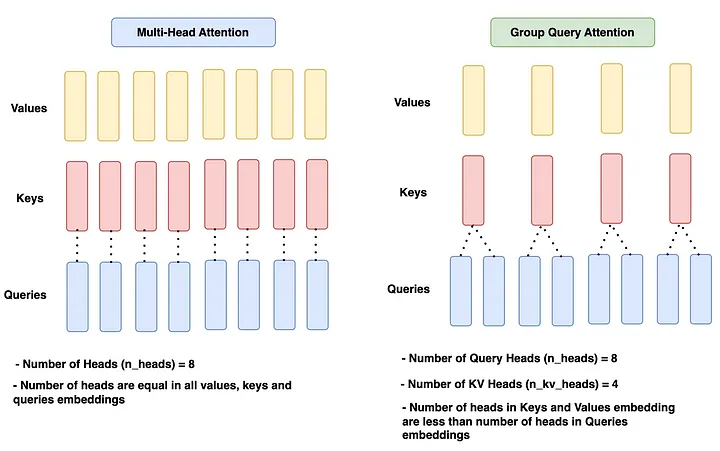
In the given diagram, the multi-head attention has an equal number of heads across all queries, keys and values which is n_heads = 8.

The Group query attention block has 8 heads for queries (n_heads) and 4- heads (n_kv_heads) for keys and values, which is 2 times less than query heads.

Since MultiHead Attention is already so good, why do we need Group query attention? To answer this, we need to go back to KV Cache for a while. The KV cache helps reduce computation resources greatly. However, as KV Cache stores more and more previous tokens, the memory resources will increase significantly. This is not a good thing for the model performance point of view as well as the financial point of view. Hence, Group query attention is introduced. Reducing the number of heads for K and V decreases the number of parameters to be stored, and hence, less memory is being used. Various test results have proven that the model accuracy remains in the same ranges with this approach.

Let’s implement this in code:

## The Attention Block [Step2c: The KV Cache; Step2d: Group Query Attention]
## As mentioned before, the naming convention follows original the meta's LLama3 GitHub

class Attention(nn.Module):
  def __init__(self, args: ModelArgs):
    super().__init__()
    self.args = args
    # Embedding dimension
    self.dim = args.dim
    # Number of heads assigned to Query
    self.n_heads = args.n_heads
    # Number of heads assigned to Key and values. If "None", the number will be same as Query.
    self.n_kv_heads = args.n_heads if args.n_kv_heads is None else args.n_kv_heads
    # Dimension of each head relative to model dimension
    self.head_dim = args.dim // args.n_heads
    # Number of repetition in order to make time Key, Value heads to match Query heads number
    self.n_rep = args.n_heads // args.n_kv_heads

    # Weight initialize for Keys, Querys, Values and Oupt. Notice that the out_feature value of weight for q and kv are based on it's heads
    self.wq = nn.Linear(self.dim, self.n_heads * self.head_dim, bias=False, device=device)
    self.wk = nn.Linear(self.dim, self.n_kv_heads * self.head_dim, bias=False, device=device)
    self.wv = nn.Linear(self.dim, self.n_kv_heads * self.head_dim, bias=False, device=device)
    self.wo = nn.Linear(self.n_heads * self.head_dim, self.dim, bias=False, device=device)

    # Initialize caches to store Key, Values at start. (KV Cache Implementation)
    self.cache_k = torch.zeros((args.max_batch_size, args.max_seq_len, self.n_kv_heads, self.head_dim), device=args.device)
    self.cache_v = torch.zeros((args.max_batch_size, args.max_seq_len, self.n_kv_heads, self.head_dim), device=args.device)

  def forward(self, x: torch.Tensor, start_pos, inference):
    # Shape of the input embedding: [bsz,seq_len,dim]
    bsz, seq_len, _ = x.shape
    # Mask will be used during 'Training' and is not required for 'inference' due to the use of KV cache.
    mask = None

    xq = self.wq(x)  #x[bsz,seq_len,dim]*wq[dim,n_heads * head_dim] -> q[bsz,seq_len,n_heads * head_dim]
    xk = self.wk(x)  #x[bsz,seq_len,dim]*wq[dim,n_kv_heads * head_dim] -> k[bsz,seq_len,n_kv_heads * head_dim]
    xv = self.wv(x)  #x[bsz,seq_len,dim]*wq[dim,n_kv_heads * head_dim] -> v[bsz,seq_len,n_kv_heads * head_dim]

    # Reshaping Querys, Keys and Values by their number of heads. (Group Query Attention Implementation)
    xq = xq.view(bsz, seq_len, self.n_heads, self.head_dim)      #xq[bsz,seq_len,n_heads, head_dim]
    xk = xk.view(bsz, seq_len, self.n_kv_heads, self.head_dim)   #xk[bsz,seq_len,n_kv_heads, head_dim]
    xv = xv.view(bsz, seq_len, self.n_kv_heads, self.head_dim)   #xv[bsz,seq_len,n_kv_heads, head_dim]

    # Model - Inference Mode: kv-cache is enabled at inference mode only.
    if inference:
      # Compute rotation matrix for each position in the sequence
      freqs_cis = precompute_freqs_cis(dim=self.head_dim, seq_len=self.args.max_seq_len * 2)
      # During inferencing, we should only take the rotation matrix range from the current position of the tokens.
      freqs_cis = freqs_cis[start_pos : start_pos + seq_len]
      # Apply RoPE to Queries and Keys embeddings
      xq, xk = apply_rotary_emb(xq, xk, freqs_cis)

      self.cache_k = self.cache_k.to(xq)
      self.cache_v = self.cache_v.to(xq)
      # Store Keys and Values token embedding into their respective cache [KV Cache Implementation]
      self.cache_k[:bsz, start_pos:start_pos + seq_len] = xk
      self.cache_v[:bsz, start_pos:start_pos + seq_len] = xv

      # Assign all the previous tokens embeddings upto current tokens position to Keys and Values variable for Attention Calculation
      keys = self.cache_k[:bsz, :start_pos + seq_len]
      values = self.cache_v[:bsz, :start_pos + seq_len]

      # At this point, they Keys and Values shape aren't same with Queries Embedding which has to be in order to computer attention score
      # Use repeat_kv function to make Keys,Values shape same as queries shape
      keys = repeat_kv(keys, self.n_rep)      #keys[bsz,seq_len,n_heads,head_dim]
      values = repeat_kv(values, self.n_rep)  #values[bsz,seq_len,n_heads,head_dim]

    # Mode - Training mode: KV-Cache not implemented
    else:
      # Compute rotation matrix and apply RoPE to queries and keys for for training.
      freqs_cis = precompute_freqs_cis(dim=self.head_dim, seq_len=self.args.max_seq_len)

      #xq[bsz,seq_len,n_heads, head_dim], xk[bsz,seq_len,n_heads, head_dim]
      xq, xk = apply_rotary_emb(xq, xk, freqs_cis)

      # Use repeat_kv function to make Keys,Values shape same as the queries shape
      #keys[bsz,seq_len,n_heads,head_dim], #values[bsz,seq_len,n_heads,head_dim]
      keys = repeat_kv(xk, self.n_rep)
      values = repeat_kv(xv, self.n_rep)

      # For training mode, we'll compute mask and apply to the attention score later
      mask = torch.full((seq_len, seq_len),float("-inf"),device=self.args.device)
      mask = torch.triu(mask, diagonal=1).to(self.args.device)

    # To compute attention, we'll need to perform a transpose operation to reshape all queries, keys and values bring heads at dim 1 and seq at dim 2
    xq = xq.transpose(1,2)                  #xq[bsz,n_heads,seq_len,head_dim]
    keys = keys.transpose(1,2)              #keys[bsz,n_heads,seq_len,head_dim]
    values = values.transpose(1,2)          #values[bsz,n_heads,seq_len,head_dim]

    # Computing attention score
    scores = torch.matmul(xq, keys.transpose(2,3)).to(self.args.device)/math.sqrt(self.head_dim)
    if mask is not None:
      scores = scores + mask

    # Apply softmax to the attention score
    scores = F.softmax(scores.float(), dim=-1).type_as(xq)
    # Matrix multiplication of attention score with the values
    output = torch.matmul(scores, values).to(self.args.device)

    # We get the contextual embedding for each head
    # All heads need to be reshaped back and combined to give a single single contextual attention output
    # Shape change: output[bsz,n_heads,seq_len,head_dim] -> output[bsz,seq_len, n_heads,head_dim] -> output[bsz,seq_len, n_heads * head_dim]
    output = output.transpose(1,2).contiguous().view(bsz, seq_len, -1)

    # shape: output [bsz,seq_len,dim]
    return self.wo(output)

# If the number of keys/values heads is less than query heads, this function expands the key/values embeddings with the required number of repetition
def repeat_kv(x:torch.Tensor, n_rep: int)-> torch.Tensor:
  bsz, seq_len, n_kv_heads, head_dim = x.shape
  if n_rep == 1:
    return x
  return (
      x[:,:,:,None,:]
      .expand(bsz,seq_len,n_kv_heads,n_rep, head_dim)
      .reshape(bsz,seq_len,n_kv_heads * n_rep, head_dim)
  )


### Test: Repeat_kv function ###
# note: xk, x_norm is already calculated during RoPE, RMSNorm testing and is being used for testing here.
# You need take out the triple quotes below to perform testing
"""
n_rep = ModelArgs.n_heads // ModelArgs.n_kv_heads
keys = repeat_kv(xk, n_rep)
print(f"xk.shape: {xk.shape}")
print(f"keys.shape: {keys.shape}")

## Test: Attention function
# You need take out the triple quotes below to perform testing

attention = Attention(ModelArgs)
x_out = attention(x_norm,start_pos=0, inference=False)
print(f"x_out.shape: {x_out.shape}")
"""
### Test Results: ###
"""
xk.shape: torch.Size([10, 256, 4, 64])
keys.shape: torch.Size([10, 256, 8, 64])
x_out.shape: torch.Size([10, 256, 512])
"""

FeedForward Network (SwiGLU Activation)

What does FeedForward Network do in the decoder block? As shown in the architecture diagram above, the attention output is first normalized during RMSNorm and then fed into the FeedForward network. Inside the feedforward network, the attention output embeddings will be expanded to the higher dimension throughout its hidden layers and learn more complex features of the tokens.

Why use SwiGLU instead of ReLU? Let’s take a look at the diagram to get the answer.

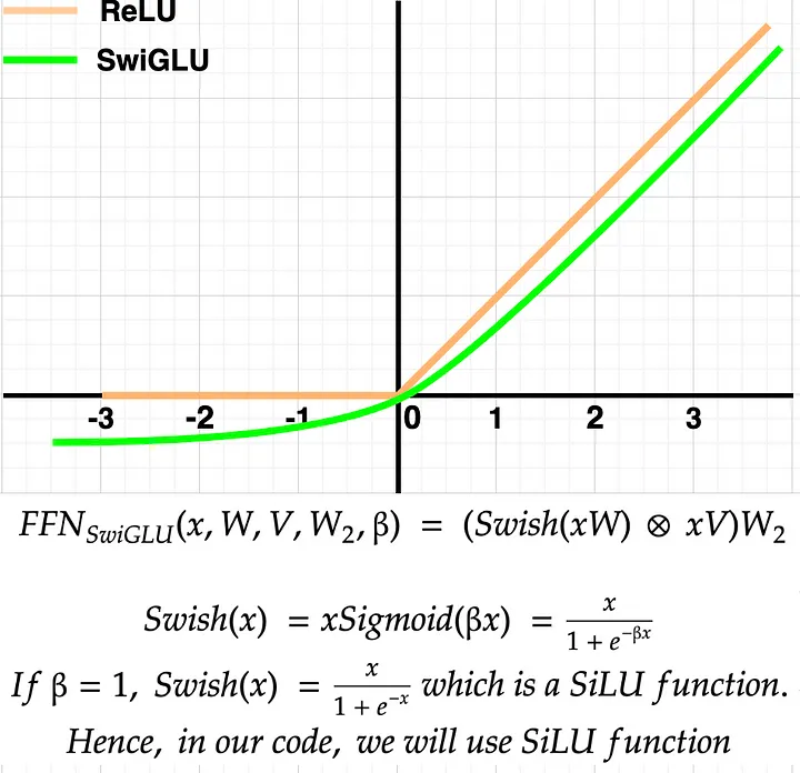
As shown in the diagram above, the SwiGLU function behaves almost like ReLU in the positive axis. However, in the negative axis, SwiGLU outputs some negative values, which might be useful in learning smaller rather than flat 0 in the case of ReLU. Overall, as per the author, the performance with SwiGLU has been better than that with ReLU; hence, it was chosen.

Let’s dive into FeedForward code:

## Step2e: The Feedfoward Network (SwiGLU activation)
class FeedForward(nn.Module):
  def __init__(self, dim:int, hidden_dim:int, multiple_of:int, ffn_dim_multiplier: Optional[float]):
    super().__init__()
    # Models embedding dimension
    self.dim = dim

    # We must use the hidden dimensions calculation shared by Meta which is the ideal one for this model
    # Hidden dimension are calculated such that it is a multiple of 256.
    hidden_dim = int(2 * hidden_dim/3)
    if ffn_dim_multiplier is not None:
      hidden_dim = int(ffn_dim_multiplier * hidden_dim)
    hidden_dim = multiple_of * ((hidden_dim + multiple_of - 1) // multiple_of)

    # define hiddne layers weights
    self.w1 = nn.Linear(self.dim, hidden_dim, bias=False, device=device)
    self.w2 = nn.Linear(hidden_dim, self.dim, bias=False, device=device)
    self.w3 = nn.Linear(self.dim, hidden_dim, bias=False, device=device)

  def forward(self, x):
    # Shape: [bsz,seq_len,dim]
    return self.w2(F.silu(self.w1(x)) * self.w3(x))



### Test: FeedForward module ###
# note: x_out is already computed at Attention testing and is being used for testing here.
# You need take out the triple quotes below to perform testing
"""
feed_forward = FeedForward(ModelArgs.dim, 4 * ModelArgs.dim, ModelArgs.multiple_of, ModelArgs.ffn_dim_multiplier)
x_out = rms_norm(x_out)
x_out = feed_forward(x_out)
print(f"feed forward output: x_out.shape: {x_out.shape}")
"""

### Test Results: ###
"""
feed forward output: x_out.shape: torch.Size([10, 256, 512])
"""

Decoder Block

As shown in the architecture diagram above (the very first diagram). The decoder block consists of multiple sub-components, which we’ve learned and coded in previous sections. Below is a pointwise operation that is being carried out inside the decoder block.

1. The embedding from the input block is fed into the Attention-RMSNorm block. This will be further fed into the Group Query Attention block.
2. The same embedding from the input block will then be added to the attention output.
3. After that, the attention output is fed into FeedFoward-RMSNorm and further fed into the FeedFoward network block.
4. The output of the FeedFoward network is then added again with the attention output.
5. The resulting output is called Decoder Output. This decoder output is then fed into another decoder block as input. This same operation will be repeated for the next 31 decoder blocks. The final decoder output of the 32nd decoder block is then passed to the Output block.

Let’s see this action in the code below:

## Step2f: The Decoder Block. The class name is assigned as TransformerBlock to match the name of Meta llama 3 code base.

class TransformerBlock(nn.Module):
  def __init__(self, args: ModelArgs):
    super().__init__()
    self.args = args
    # Initilizate RMSNorm for attention
    self.attention_norm = RMSNorm(dim=args.dim, eps = args.norm_eps)
    # Initilizate Attention class
    self.attention = Attention(args)
    # Initilizate RMSNorm for feedfoward class
    self.ff_norm = RMSNorm(dim=args.dim, eps = args.norm_eps)
    # Initilizate feedfoward class
    self.feedforward = FeedForward(args.dim, 4 * args.dim, args.multiple_of, args.ffn_dim_multiplier)

  def forward(self, x, start_pos, inference):
    # start_pos = token position for inference mode, inference = True for inference and False for training mode
    # i) pass input embedding to attention_norm and then pass to attention block.
    # ii) the output of attention is then added to embedding(before norm)
    h = x + self.attention(self.attention_norm(x), start_pos, inference)

    # i) pass attention output to ff_norm and then pass to the feedforward network.
    # ii) the output of feedforward network is then added to the attention output(before ff_norm)
    out = h + self.feedforward(self.ff_norm(h))
    # Shape: [bsz,seq_len,dim]
    return out


### Test: TransformerBlock ###
# You need take out the triple quotes below to perform testing
"""
x = torch.randn((ModelArgs.max_batch_size, ModelArgs.max_seq_len, ModelArgs.dim), device=device)
transformer_block = TransformerBlock(ModelArgs)
transformer_block_out = transformer_block(x,start_pos=0, inference=False)
print(f"transformer_block_out.shape: {transformer_block_out.shape}")
"""

### Test Results: ###
"""
transformer_blo

Step 3: The Output Block

The decoder output of the final decoder block will feed into the output block. It is first fed into the RMSNorm. Then, it will feed into the Linear Layer which generates logits. Next, one of the following two operations happens.

• If the mode is inference, top_p probability is calculated and the next token is generated. The next tokens generated will stop if the max generation length is reached or the end of sentence token is generated as the next token.
• If the mode is Training, loss is computed with the target labels and training is repeated till the max epochs length is reached.

Let’s take a look at the output block flow diagram for more clarity.

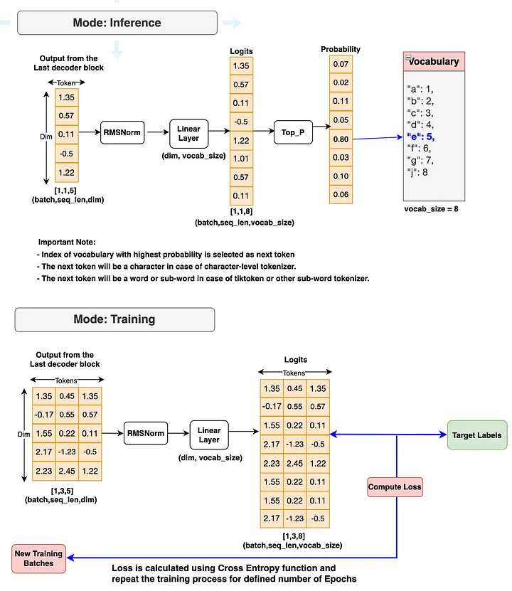
Finally, let’s combine all components of 3 blocks (input block, decoder block and output blocks. This gives our final Llama 3 model.

## Step3: The Output Block
# This is the Llama 3 model. Again, the class name is maintained as Transformer to match with Meta Llama 3 model.

class Transformer(nn.Module):
  def __init__(self, params: ModelArgs):
    super().__init__()
    # set all the ModelArgs in params variable
    self.params = params
    # Initilizate embedding class from the input block
    self.tok_embeddings = nn.Embedding(params.vocab_size, params.dim)

    # Initialize the decoder block and store it inside the ModuleList. 
    # This is because we've 4 decoder blocks in our Llama 3 model. (Official Llama 3 has 32 blocks)
    self.layers = nn.ModuleList()
    for layer_id in range(params.n_layers):
      self.layers.append(TransformerBlock(args=params))

    # Initilizate RMSNorm for the output block
    self.norm = RMSNorm(params.dim, eps = params.norm_eps)
    
    # Initilizate linear layer at the output block.
    self.output = nn.Linear(params.dim, params.vocab_size, bias=False)

  def forward(self, x, start_pos=0, targets=None):
    
    # start_pos = token position for inference mode, inference = True for inference and False for training mode
    # x is the batch of token_ids generated from the texts or prompts using tokenizers.
    # x[bsz, seq_len] -> h[bsz, seq_len, dim]
    h = self.tok_embeddings(x)

    # If the target is none, Inference mode is activated and set to "True" and "False" if Training mode is activated.
    if targets is None:
      inference = True
    else:
      inference = False

    # The embeddings (h) will then pass though all the decoder blocks.
    for layer in self.layers:
      h = layer(h, start_pos, inference)

    # The output from the final decoder block will feed into the RMSNorm
    h = self.norm(h)

    # After normalized, the embedding h will then feed into the Linear layer. 
    # The main task of the Linear layer is to generate logits that maps the embeddings with the vocabulary size.
    # h[bsz, seq_len, dim] -> logits[bsz, seq_len, vocab_size]
    logits = self.output(h).float()
    loss = None

    # Inference mode is activated if the targets is not available
    if targets is None:
      loss = None
    # Training mode is activated if the targets are available. And Loss will be calculated for further model training. 
    else:
      loss = F.cross_entropy(logits.view(-1, self.params.vocab_size), targets.view(-1))

    return logits, loss


### Test: Transformer (Llama Model) ###
# You need take out the triple quotes below to perform testing
"""
model = Transformer(ModelArgs).to(ModelArgs.device)
print(model)
"""

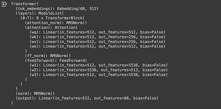
The Llama 3 model we’ve just built looks perfect. We’re now ready to start our training process.

Step 4: Train our Llama 3 Model

The training flow is provided in the output block flow diagram (step 3). Please refer to that flow again if you would like to have more clarity before starting training. Let’s begin writing the training code. I’ll also provide the necessary explanation within the code block as well.

## Step 4: Train Llama 3 Model:

# Create a dataset by encoding the entire tiny_shakespeare data token_ids list using the tokenizer's encode function that we've built at the input block section
dataset = torch.tensor(encode(data), dtype=torch.int).to(ModelArgs.device)
print(f"dataset-shape: {dataset.shape}")

# Define function to generate batches from the given dataset
def get_dataset_batch(data, split, args:ModelArgs):
  seq_len = args.max_seq_len
  batch_size = args.max_batch_size
  device = args.device

  train = data[:int(0.8 * len(data))]
  val = data[int(0.8 * len(data)): int(0.9 * len(data))]
  test = data[int(0.9 * len(data)):]

  batch_data = train
  if split == "val":
    batch_data = val

  if split == "test":
    batch_data = test
  
  # Picking random starting points from the dataset to give random samples for training, validation and testing.
  
  ix = torch.randint(0, len(batch_data) - seq_len - 3, (batch_size,)).to(device)
  x = torch.stack([torch.cat([token_bos, batch_data[i:i+seq_len-1]]) for i in ix]).long().to(device)
  y = torch.stack([torch.cat([batch_data[i+1:i+seq_len], token_eos]) for i in ix]).long().to(device)
  
  return x,y

### Test: get_dataset function ###
"""
xs, ys = get_dataset_batch(dataset, split="train", args=ModelArgs)
print([(decode(xs[i].tolist()), decode(ys[i].tolist())) for i in range(len(xs))])
"""

# Define a evaluate loss function to calculate and store training and validation loss for logging and plotting
@torch.no_grad()
def evaluate_loss(model, args:ModelArgs):
  out = {}
  model.eval()

  for split in ["train", "val"]:
    losses = []
    for _ in range(10):      
      xb, yb = get_dataset_batch(dataset, split, args)
      _, loss = model(x=xb, targets=yb)
      losses.append(loss.item())
    out[split] = np.mean(losses)

  model.train()
  return out

# Define a training function to perform model training
def train(model, optimizer, args:ModelArgs):
    epochs = args.epochs
    log_interval = args.log_interval
    device = args.device
    losses = []   
    start_time = time.time()

    for epoch in range(epochs):
        optimizer.zero_grad()
        
        xs, ys = get_dataset_batch(dataset, 'train', args)
        xs = xs.to(device)
        ys = ys.to(device)
        logits, loss = model(x=xs, targets=ys)
        loss.backward()
        optimizer.step()

        if epoch % log_interval == 0:
            batch_time = time.time() - start_time
            x = evaluate_loss(model, args)
            losses += [x]            
            print(f"Epoch {epoch} | val loss {x['val']:.3f} | Time {batch_time:.3f}")
            start_time = time.time()
    
    # Print the final validation loss
    print("validation loss: ", losses[-1]['val'])
    # Display the interval losses in plot 
    return pd.DataFrame(losses).plot()

Now, that we’ve defined the training function. Let’s start training with the following code block and observe the training results in the plot once the training is completed.

## Start training our Llama 3 model
model = Transformer(ModelArgs).to(ModelArgs.device)
optimizer = torch.optim.Adam(model.parameters())

train(model, optimizer, ModelArgs)

The above image displays the training and validation loss graph. The training has been conducted over 2500 epochs. It took around 10 min to complete the training process using Google Colab with default GPU and RAM settings which is very fast. The validation loss at the final epoch is 2.19 which is considered okay given the amount of training data we’re using and the number of epochs. To reduce the losses significantly, we will have to increase the size of the training data, higher number of epochs and higher GPU or processing power.

Now that we’ve completed our training. Let’s head into our final step — Inference and see how well the model generates the output texts given new input prompts.

Step 5: Inference Llama 3 Model

The inference flow is provided in the output block flow diagram(step 3). Let’s begin writing the inference code.

## Step 5: Inference Llama 3 Model:
# This function generates text sequences based on provided prompts using the LLama 3 model we've built and trained.

def generate(model, prompts: str, params: ModelArgs, max_gen_len: int=500, temperature: float = 0.6, top_p: float = 0.9):

    # prompt_tokens: List of user input texts or prompts
    # max_gen_len: Maximum length of the generated text sequence.
    # temperature: Temperature value for controlling randomness in sampling. Defaults to 0.6.
    # top_p: Top-p probability threshold for sampling prob output from the logits. Defaults to 0.9.
    # prompt_tokens = [0]
    bsz = 1  #For inferencing, in general user just input one prompt which we'll take it as 1-batch
    prompt_tokens = token_bos.tolist() + encode(prompts)
    assert len(prompt_tokens) <= params.max_seq_len, "prompt token length should be small than max_seq_len"
    total_len = min(len(prompt_tokens)+max_gen_len, params.max_seq_len)   

    # this tokens matrix is to store the input prompts and all the output that is generated by model.
    # later we'll use the tokenizers decode function to decode this token to view results in text format
    tokens = torch.full((bsz,total_len), fill_value=token_pad.item(), dtype=torch.long, device=params.device)

    # fill in the prompt tokens into the token matrix
    tokens[:,:len(prompt_tokens)] = torch.tensor(prompt_tokens, dtype=torch.long, device=params.device)

    #create a prompt_mask_token for later use to identify if the token is a prompt token or a padding token
    # True if it is a prompt token, False if it is a padding token
    input_text_mask = tokens != token_pad.item()

    #now we can start inferencing using one token at a time from the prompt_tokens list starting with the first position.
    prev_pos = 0
    for cur_pos in range(1, total_len):
      with torch.no_grad():
        logits, _ = model(x=tokens[:,prev_pos:cur_pos], start_pos=prev_pos)
      if temperature > 0:      
        probs = torch.softmax(logits[:, -1]/temperature, dim=-1)
        next_token = sample_top_p(probs, top_p)        
      else:
        next_token = torch.argmax(logits[:, -1], dim=-1)        

      next_token = next_token.reshape(-1)

      # only replace the token if it's a padding token
      next_token = torch.where(input_text_mask[:, cur_pos], tokens[:, cur_pos], next_token)
      tokens[:, cur_pos] = next_token

      prev_pos = cur_pos
      if tokens[:,cur_pos]==token_pad.item() and next_token == token_eos.item():
        break

    output_tokens, output_texts = [], []    

    for i, toks in enumerate(tokens.tolist()):
      # eos_idx = toks.index(token_eos.item())
      if token_eos.item() in toks:
        eos_idx = toks.index(token_eos.item())
        toks = toks[:eos_idx]

      output_tokens.append(toks)
      output_texts.append(decode(toks))
    return output_tokens, output_texts

# Perform top-p (nucleus) sampling on a probability distribution.
# probs (torch.Tensor): Probability distribution tensor derived from the logits.
# p: Probability threshold for top-p sampling.
# According to the paper, Top-p sampling selects the smallest set of tokens whose cumulative probability mass exceeds the threshold p. 
# The distribution is renormalized based on the selected tokens.
def sample_top_p(probs, p):
    probs_sort, prob_idx = torch.sort(probs, dim=-1, descending=True)
    probs_sum = torch.cumsum(probs_sort, dim=-1)
    mask = probs_sum - probs_sort > p
    probs_sort[mask] = 0.0
    probs_sort.div_(probs_sort.sum(dim=-1, keepdim=True))
    next_token = torch.multinomial(probs_sort, num_samples=1)
    next_token = torch.gather(prob_idx, -1, next_token)    
    # Sampled token indices from the vocabular is returned 
    return next_token

Let’s perform inferencing on new Prompts and check the generated output

## Perform the inferencing on user input prompts
prompts = "Consider you what services he has done"
output_tokens, output_texts = generate(model, prompts, ModelArgs)
output_texts = output_texts[0].replace("<|begin_of_text|>", "")
print(output_texts)

## Output ##
"""
Consider you what services he has done o eretrane
adetranytnn i eey i ade hs rcuh i eey,ad hsatsTns rpae,T
eon o i hseflns o i eee ee hs ote i ocal ersl,Bnnlnface
o i hmr a il nwye ademto nt i a ere
h i ees.
Frm oe o etrane o oregae,alh,t orede i oeral
"""

And yes, we can see that our Llama 3 model is able to perform inference and generate texts on new prompts, though the output does not seem great given the amount of training data and epochs we’ve used for training. I am sure with much larger training data, we’ll achieve much better accuracy.

And this is it! we have successfully built our own Llama 3 model from scratch. We’ve also successfully trained the model and managed to perform inferencing to generate new texts within a very short amount of time using Google Colab Notebook with given free GPU and RAM. If you have followed along so far, I would personally congratulate you for the great effort you’ve put in.

My final thoughts

Llama 3 and its other variances are the most popular open-source LLM currently available in the LLM space. I believe the ability to build Llama 3 from scratch provides all the necessary foundation to build a lot of new exciting LLM-based applications. I truly believe that knowledge should be free to all. Feel free to use the source code and update it to build your personal or professional projects. Good luck to you all.

References

Meta Llama3 Github: https://github.com/meta-llama/llama3